“Undoing” an SVN revision

This is the second in a series of posts I began this summer and didn’t have time to finish.

Edit 2011/01/17: I finally noticed and fixed a small glitch in the raw command line I was using, probably caused by my use of “<>” in the example text. Sorry, folks.

We all know how it feels, right? You’ve been coding away happily, decide it’s time to push everything to your version control system of choice, type out a brilliant commit message, and hit Enter–only to find out five seconds later that you just committed something you shouldn’t have committed and everyone else is in trouble when they happen to update. What do you do now?

Well, if you have a decent version control system (VCS) such as Mercurial or Git, you take advantage of the built-in undo or undo-like command and simply undo your commit. Most modern distributed VCS’s have one, giving you at least one chance to fix your work before you hand it out for everyone else to use. However, some less-than-fun VCS’s make it difficult (mostly because they’re designed to keep the information you give them forever, warts and all, which is not a bad thing). However, it’s still usually possible to fake an undo.

Take Subversion, for example. It’s not my favorite VCS for reasons I may go into later, but it’s still a very solid one if you like and/or need the centralized type of thing. I used it a lot this summer while doing an internship with Sentry Data Systems, and I found myself needing to rollback a commit on some files a time or two. So, I did some research.

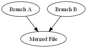
Graphical representation of a merge

Arguably the best way to rollback a commit in Subversion is to perform what they call a reverse-merge. In a normal merge, you take two versions of a file, compare them to figure out what’s different between them, and then create a new file containing the consensus content of both files (see picture to the right).

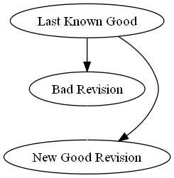
Graphical representation of a reverse merge

In a reverse-merge, you figure out what changes were made in a given revision, and then commit a new revision that reverts all of those changes back to the version before you committed your bad revision (see picture to the right), which means your bad revision will be simply skipped over as far as your comrades are concerned. Subversion provides a simple series of commands for this:

svn merge -c -{bad revision number} [{files to revert}]

Here’s how it works.

  1. The svn merge portion of the command basically tells Subversion you want to merge something. svn is the command-line tool to interact with a Subversion repository, and merge…well, you get the idea.
  2. -c -{bad revision number} tells Subversion that we want to work with the changes related to the revision numbered {bad revision number}. In this case, since we’re passing in a negative sign in front, we’re saying we want to remove those changes from the working directory. If you left out that negative sign, you’d actually pull the changes from that revision into the current working directory, which is usually only useful if you’re cherry-picking across branches. Whether that’s a good idea or not is left to the reader.
  3. [{files to revert}] are an optional list of files to undo changes in. Basically, if you pass in a list of files here, only those files will have their changes from revision–any other files changed in that revision will not be affected.

That’s pretty much it. Once you run that command (assuming there are no conflicts in your merge), you will be able to simply commit (with a helpful commit message, of course) and everything will be back to normal–your comrades in arms will be able to keep working without the overhead of your bad commit cluttering up their working environment, which is always a good thing.
Tar Pipe

This is the first in a series of posts I began this summer and only now have time to finish.

Every once in a while, I find myself needing to copy a large number of files from one Linux machine to another, ideally as fast as possible.  There are a lot of ways to do this, but the most common method usually goes something like this:

  • Tar everything up (with some form of compression if your network connection is slow).
  • (S)FTP/SCP  the file to the new server.
  • Move the file to the new location, making directories as needed.
  • Extract the tar file into the new directory.

This is all well and good, and it tends to work well in most cases–it’s just kind of laborious.  I prefer a simpler method that basically wraps everything up into a single step, affectionately known as a tar pipe.  The (admittedly somewhat complex) command follows.

  SRCDIR=  # fill in with your source directory
  DESTDIR= # fill in with your destination directory--note that your
           # uploaded directory will appear inside this one
  USER=    # fill in the your remote user name
  HOST=    # fill in with your remote host name
  tar -cvzf - $SRCDIR | ssh $USER@$HOST "mkdir -p $DESTDIR; tar -xz -C $DESTDIR

The variables are just to make things a little more easy to read (feel free to ignore them if you like), and I do recommend using a full path for the DESTDIR directory, but the basic process is ridiculously easy.  Here’s the breakdown on how the whole thing works.

  1. The tar -cvzf - $SRCDIR very obviously tars everything up, just like you normally would.  The key difference from the normal tar procedure is the fact that the “file” you’re creating with tar is actually sent to stdout (by the -f - option) instead of being written to the file system.  We’ll see why later.
  2. The | (pipe) passes everything on stdout on as stdin for the next command, just like normal.
  3. The ssh command is the fun part.
    1. We start an ssh session with $HOST as $USER.
    2. Once that’s established, we run two commands.
      1. mkdir -p $DESTDIR to make the destination directory, if needed.
      2. tar -xz -C $DESTDIR to untar something. What, we’re not sure yet.

What it untars is a bit of a mystery, as we don’t really tell it what it’s supposed to work on.  Or do we?  As it turns out, ssh passes whatever it receives on stdin on to the command it runs on the server.  I.e., all that stuff we just tar’red up gets passed along through the magic of piping from the local machine to the remote machine, then extracted on the fly once it gets to that machine.

You can see the benefit of this, I trust–instead of that whole four command process we detailed above, including manually logging into the remote server to actually extract the new file, we have one fairly simple command that handles taring, uploading, and extracting for us, with the added benefit of not requiring us to actually create any files we don’t have to create.  That’s kind of cool, right?

Note:  I’ve seen other implementations of the tar pipe, but this is the one I’ve used been using recently.  It’s worked for me on Red Hat 5, but your mileage may vary.

RAMMCAP: CD-HIT and ORF_FINDER

This is the second part of a series of posts on the RAMMCAP suite of bioinformatics tools.

Last time, we left off with a freshly compiled version of RAMMCAP ready for testing.  Like last time, we’ll start with the README in the current directory, which is the rammcap directory inside the main directory (named RAMMCAP-20091106 in my case) from the RAMMCAP download.

The new README has its own test script, so I’m going to follow this one. The first thing to run is the CD-HIT-EST program.

CD-HIT-EST

The CD-HIT-EST program is the clustering program. It takes in a FASTA-formatted file and clusters that data according to a greedy algorithm that uses simple word counting and indexing to help speed things up considerably. Basically, it:

  1. Sorts the sequences from longest to shortest.
  2. Begins clustering:
    1. Compare the current sequence to the list of known clusters.
      1. If it matches an existing cluster, it is added to that cluster and made the “representative” sequence for that cluster if it is longer than the existing “representative” sequence.
      2. If it doesn’t match an existing cluster, a new cluster is made with this sequence as the representative sequence.
    2. Repeat until all the sequences are clustered.

(None of which I knew at the time I ran this for the first time, but it’s information that makes sense here.)

I pull out the really long test command (written below), prepare myself, and hit Enter. It takes a long time to complete.

../cd-hit/cdhit-est -i testdb -o testdb_95 -M 50 -B 1 -d 0 -n 10 
     -l 11 -r 1 -p 1 -g 1 -G 0 -c 0.95 -aS 0.8 > testdb_95.log

While that’s going, here’s what that command means:

  • ../cd-hit/cd-hit-est – use the CD-HIT-EST command, which is the CD-HIT command for DNA/RNA comparison tasks. The original CD-HIT was written for protein comparison.
  • -i testdb – use the testdb file as the input file. This file is a FASTA file with 1,000,000 sequences at most 361 bases long pulled from various metagenomic samples by the author.
  • -o testdb_95 – write the output to a file called testdb_95
  • -M 50 – I have 50 MB of RAM free (which I don’t think really makes sense, but that’s what the README says)–turns out it’s actually the maximum available memory, not the amount of free memory according to the rest of the documentation.
  • -B 1 – sequences are stored on the hard drive (1) instead of in RAM (0)
  • -d 0 – The length of the description in .clster file. Since it’s 0, it just takes the FASTA sequence description up to the first space.
  • -n 10 – the word length
  • -l 11 – length of the throw_away_sequences
  • -r 1 – compare both strands of DNA
  • -p 1 – print the alignment overlap in the .clstr file (if 0, it’s not printed)
  • -g 1 – clusters the strings into the most similar cluster, not the first one CD HIT finds, which is the default (0).
  • -G 0 – don’t use global sequence identity, i.e., treat each input sequence individually when calculating identity.
  • -c 0.95 – cluster at 95% sequence identity
  • -aS 0.8 – alignment coverage for the shorter sequence. In this case, it means that the alignment between the longer and shorter sequence must cover at least 80% of the shorter sequence.
  • > testdb_95.log – write the standard output to the testdb_95.log file
  • There are other options available, which I’m not going to go into much for right now.

Long story short, it takes around 200 minutes to complete its test data processing. That’s roughly 3 hours and 20 minutes, which I think is pretty long for a test, though I did limit the amount of memory it could use to 50 MB–upping that limit will probably speed things up substantially, but according to what I read in the README I couldn’t. In retrospect, though, I think upping the limit is just fine, especially with the information I’m reading in the other files. (UPDATE: Upping the memory limit to 400MB, the default, drops the execution time down to about 67 minutes. Eight fold memory increase, three fold time decrease–not great, but not too shabby.)

ORF_FINDER

The next program to run is the ORF_FINDER. This program apparently is a program to scan the sequences for ORFs (not surprising given the name), which are what most people mean when they talk about their “genes” and their DNA (kind of).

../orf_finder/orf_finder -l 30 -L 30 -t 11  -i testdb -o testorf

This command takes far fewer options.

  • ../orf_finder/orf_finder – runs the orf_finder command.
  • -l 30 – the minimal length of the ORF.
  • -L 30 – the minimal length of the ORF between stop codons. I’m not sure exactly how this differs from the -l option. Maybe you need to move at least 30 bases past the end of the previous stop codon before starting to look for another stop codon?
  • -t 11 – Translation table?. Again, not sure what this represents.
  • -i testdb – Use the testdb file as input.
  • -o testorf – Write the output to the testorf file.
  • Again, there are other options I’m not going to talk about much.

In addition to having far fewer options, ORF_FINDER takes far less time to execute. Roughly a minute and a half on the same dataset, which is a pretty huge upgrade. ORF finding is a much simpler task than sequence clustering, obviously. Now for the fun part–clustering the ORFs with the real CD-HIT program.

CD-HIT

Now, CD-HIT works basically the same way that CD-HIT-EST does, except it scans for amino acids instead of nucleotides. The full commands I’m running are:

../cd-hit/cdhit -i testorf -o testorf_95 -M 400 -d 0 -n 5 -p 1 
     -g 1 -G 0 -c 0.95 -aS 0.8 > testorf_95.log
../cd-hit/cdhit -i testorf_95 -o testorf_60 -M 400 -d 0 -n 4 -p 1 
     -g 1 -G 0 -c 0.60 -aS 0.8 > testorf_60.log
../cd-hit/clstr_rev.pl testorf_95.clstr testorf_60.clstr 
     > testorf_60full.clstr

It has much the same options as CD-HIT-EST, so I’m not going go into a huge amount of detail on those. Instead, notice how I’m going to:

  1. Cluster the ORFS at 95% identity.
  2. Re-cluster the ORFs with less stringent criteria (60% identity and a shorter word length) to help cluster the non-redundant sequences.
  3. Combine the two clustering runs into a single cluster file.

Running things this way (according to the documentation) can help generate a sort of hierarchical structure of clusters. This makes sense, since the ones at 95% identity at the very least are closely related and may actually be redundant sequences while those at 60% are more distant relatives and may be homologs from divergent species or something similar.

The first run of CD-HIT took around 98 minutes, roughly an extra half an hour than just clustering the sequences as a whole. I’m guessing that since the ORFs are more similar to each other than just the sequences as a whole that they take longer to cluster.

The second run of CD-HIT took around 235 minutes, probably because the less stringent criteria took longer to process. Combining the two cluster files only took around 15 seconds, so at least that’s an easy task.

That takes care of the basic tools included with RAMMCAP.  I’ll explore some of the graphical tools in a later post.

RAMMCAP: Introduction, Download, and Install

This is the first part of a series of posts on the RAMMCAP suite of bioinformatics tools.

The Rapid Analysis of Multiple Metagenomes with a Clustering and Annotation Pipeline (RAMMCAP) is a tool used for analysis of metagenomic data. What it does is try to cluster and functionally annotate a set of metagenomic data, which means it takes the data, groups like pieces of data together into clusters, and then tries to figure out what the various clusters do. It’s made up of several tools, only two of which I’ve actually used and I’ll talk about later. Camera, the organization behind RAMMCAP, provides a web service where you can use RAMMCAP without installing it, but it has data limits that I’ll break very easily with my datasets plus they require registration, which seems non-functional right now (at least, I can’t get a new account set up and I’ve tried several times over the course of the last few days). So, I downloaded it a few weeks ago and worked on getting it to run over the course of several days.  This post, and the others in this series, is a record of that process, including some initial miss-steps.  If you have any questions or see other places where I stepped wrongly, leave a comment and let me know.

First Impressions

First off, the RAMMCAP download (found on the page linked above) is huge–the source code alone was a roughly 760 MB download, which extracts to around 3 gigs. That three gigs might contain some duplicate data–the folder structure is pretty disorganized and a casual glance shows a lot of folders with the same names. There are a lot of symlinks, though, so I could be wrong there. (The more I see, the more I’m convinced I’m right, though.)

Second, it looks like the source bundled a bunch of tools along with the main RAMMCAP code, including versions of BLAST, HMMER, and Metagene. That added a lot to the bulk of the download (roughly 450 MB). There’s also a huge amount of data here, including a version of the Pfam and TIGRFAM libraries (772 and 444 MB, respectively), and a couple other tools I haven’t heard of before that might be part of RAMMCAP.

Compiling, Phase 1

The README file in the main directory contains basic information on how to compile some of the tools including CD-HIT, ORF_FINDER, and CD-HIT-454, as well as the HMMERHEAD extension to the HMMER, which is optional. The instructions are pretty basic–just do the standard “make clean;make” and things should be good. I wrote a little build script to handle this, just in case I need to do this again for some reason. Everything seems to build fine with the exception of HMMERHEAD, but I’m just going to ignore that for now. Time for testing this puppy out.

Testing, Phase 1

The README indicates that there should be an examples folder somewhere with some basic test data I can use, but I don’t see it anywhere. Looking around…not seeing it. Turns out, it’s inside the rammcap directory inside the main directory.

Compiling, Phase 2

Inside the rammcap directory, I find a new README with some major differences from the one outside this directory, plus what looks like symlinks with the same names as some of the directories outside. Looks like they point to the same directories as the other ones, but I’ll recompile things, anyway, just in case. Good thing I wrote that build script.

Except that the build instructions aren’t the same–I don’t have to build CD-HIT-454, but I do need to make sure gnuplot and ImageMagick are installed. They are, which is good, because I’d either have to contact one of the tech guys to install it on this machine or I’d have to install it to my user directory, which I’ve done with several tools I need or don’t want to do without. Once I pull out that CD-HIT-454 reference, the build works fine.

Since my second round of testing was a much larger task, I’ll leave that for a later post.

I’m back! (Part 2)

One other thing I’m going to try to use this blog for is to help me keep track of some of the tools I’m using for an RA project this year.  (“RA” in the “Research Assistant” sense, not the “Resident Advisor” sense.)  I’m studying metagenomics under Yuzhen Ye, specifically the automated functional prediction based on phylogenetic profiling (which is a fancy way of saying I want to figure out what the various pieces I’m working with do by comparing them with related genes in other organisms for which we know the function).

Needless to say, this new responsibility requires me to use a lot of tools that I’ve never heard of before, and I’ll feature some of them here, mainly so I can summarize the way they work and the way one uses them without having to refer back to the documention (which often is unclear, confusing, incomplete, or over-complicated).  Hopefully other people who come along after me can use these little tutorials and save themselves some time figuring things out.  I’m going to start out with a tool called RAMMCAP.