Strange Loop 2010: Thursday

Last week, I spent Thursday and Friday at the Strange Loop conference in St. Louis, Missouri.  It turned out to be a pretty great conference, even if I missed out on a lot of interesting talks due to a school project I had to finish and a lot of time spent volunteering.  The ones I did make it to were amazing, however.  (You can access the slides for each of the talks at the Strange Loop presentations page).

Thursday

I started off with Hilary Mason‘s talk on machine learning, and even through I missed the first 10-15 minutes or so, I arrived in time to hear her (a) run through Bayes’ Theorem in about a minute without going too far over the audience’s heads (or so I thought), (b) give a high-level overview of her Twitter Commander (Github link) Python application (which uses machine learning techniques to filter tweets from the 640 people she follows on Twitter) (c) say “Cheat as much as you can” in regards to solving difficult problems (which is basically one of my own programming mantras) and (d) mention both of my machine learning textbooks (Machine Learning by Thomas Mitchell and Pattern Recognition and Machine Learning by Christopher Bishop) casually in the Q&A session after her talk.  Not bad for only catching 45 minutes or so of her talk.

Then, I had to take a hiatus to finish up my project proposal for, ironically enough, my Machine Learning class.  That took a while.

The next session I attended was by Kyle Simpson, better known as Getify in the webdev world.  (I hadn’t heard of him, but it’s a big place and I’ve been out of the loop for a while.)  He gave a talk promoting using Javascript for what he referred to as the “middle end” of webapp development–the part of the webapp where the browser code meets the server code.  The basic idea is rooted in the DRY (Don’t Repeat Yourself) principle–rewriting code is bad, but when writing web applications, we typically use two different programming languages (one on the client, one on the server) and repeat ourselves all over the place.  Getify’s premise is that since we can’t run PHP, ASP, or any other server-side language in the browser, we should change the server to run the browser’s language, Javascript.  He actually built a proof of concept JS-based server from the V8 Javascript engine called BikehainJS (Github link).  He built a basic, but functional URL shortener called shortie.me using BikechainJS and walked us through the basic code behind the app.  Pretty cool stuff, and I like the idea, though I think he’s got a long way to go to get this off the ground.

The next talk I heard was on Clojure‘s solution to the Expression Problem by Chris Houser (or Chouser, as I knew him at Sentry Data Systems), co-author of the new The Joy of Clojure book.  The Expression Problem is kind of complicated (I’m still not sure I understand all the nuances), but the basic idea is that when we try to make an existing data type do something it’s not meant to do (to “express” a new trait), there are major issues.  Chouser’s example involved extending two custom classes (which we have complete control over) with methods to display themselves in a report, and then trying to back-port those display methods to built-in classes (such as Vectors in Java–see his talk for full details, because I’m glossing over a lot).  Most languages provide some way to do this (wrapper classes, monkey patching), but Clojure has a couple of really cool methods called multimethods and protocols.  Multimethods are a sort of function overloading while protocols feel like advanced monkey patching with some extra safeguards.  While those methods are cool, I think I’ll stick with monkey patching since the languages I use most often don’t have those tricks and I haven’t run into any of monkey patching’s problems.  (Yet.)

The last talk on Thursday was by Guy Steele, one of the original Lisp hackers and one of the original authors of the Jargon File, along with numerous other things.  His talk was on parallel programming and how not to do it.  After a long breakdown of a program he wrote on a punch card (which was fascinating and hugely relevant to the talk, but probably a little on the long side), he introduced a pretty simple idea:  instead of manually mucking around with the details of parallel programming (analogous to what he had to do with his punch card), why don’t we just let the compiler figure it out? We already let the compiler (or really low level libraries) do most of the really annoying work like register management, anyway (unless we’re writing C or C++), and the compilers do a great job, much better than most people can do and tremendously faster.  Why can’t we do that with parallel programming?  We have to be a little smarter about how we design programs in the first place, and many (if not all) of the tricks we’ve been learning for the past 50 years or so no longer work, but the benefits are usually worth it in the long run, except for the smallest of toy programs.  Once we’ve done the high-level work for the compiler, which it can’t do, we let it handle the nitty-gritty details of the memory and processor management.  While Steele made his case, he also introduced his current work at Sun Labs:  a programming language called Fortress where running code in parallel is almost trivial (so long as you design it right from the beginning, which is usually the problem).  It does show a ton of potential and is really very cool–Fortress is definitely on my list of languages to check out.

Ok, that’s enough for now, as this post is getting quite long.  I’ve covered all the talks I saw on Thursday, so now is a good time to take a break.  I’ll finish up the talks from Friday later this week.
Article Summary: Island Biogeography Reveals the Deep History of SIV

A couple of weeks ago, I ran across an article in the New York Times on some recent discoveries that totally rewrote the known history of HIV.  Needless to say, I was intrigued.  The article was actually about simian immunodeficiency virus (or SIV), the precursor for HIV that affects other primates.  It is thought that SIV crossed into humans (thus becoming HIV) sometime in the early part of the 20th century, though the exact time frame isn’t known.

According to the NYT article, the scientific community thought that SIV was a relatively new virus, emerging in primates sometime in the last few hundred years, and that this new research basically trumps that idea.  However, that’s only half the story, as you’ll discover if you actually read the paper presenting the research, which was published in Science on September 17 of this year.

In the paper, Worobey, et al.,  (the authors) set out to clear up the history of SIV.  It turns out there were two competing theories for the evolution of SIV, one being the few centuries version mentioned in the NYT article.  The other theory, which the new research supports, basically just said that SIV was old–probably very old, as some research suggests that similar viruses arose as much as 14 million years ago (see http://www.pnas.org/content/105/51/20362).

To solve this mystery, Worobey, et al., looked into six monkey species from Bioko Island, an island that separated from mainland Africa 10-12 thousand years ago.  Interestly enough, they found 4 species-specific strains of SIV.  Each of those monkey species (the red-eared guenon, the black colobus, the drill, and Preuss’s guenon) has a relative on the mainland that also possesses a strain of SIV, which makes it relatively easy to build a phylogenetic tree to help figure out just how long ago the strains split off from each other.

From what Worobey, et al., discovered, some strains of SIV have been around approximately 33,000 years ago, and quite possibly as much as 133,000. Here’s how.

  1. Ignoring the possibility of human contamination, we know that the island strains diverged from their mainland counterparts at least 10,000 years ago, since that’s when the island became an island.
  2. They then used amino acid sequence differences to estimate the most recent common ancestor (TMRCA) of the SIV variants.  (Presumably using standard methods to make the estimates, but it’s not spelled out how they get their figures.)  That gives us our estimate for sequence divergence roughly 77,000 years ago, with a 95% confidence interval ranging from ~33,000 to ~133,000 years ago.
  3. They repeated their analysis using nucleotide  differences and third codon differences.  Each of those estimates came in much lower than the amino acid estimate (though still considerably more than the supposed SIV age of a few hundred years–so much for that theory).

So, why is this important?  The authors give two main reasons.

  1. If we’ve just pushed back the origin of SIV 33 thousand years or more, what does that mean for HIV, which we think only arose about 100 years ago?  Could that also have an even longer history than we can even imagine right now?  We should investigate.
  2. We now know (or are extremely confident) that SIV is ancient, giving its hosts thousands of years to adapt to its effects.  This probably explains why monkeys infected with SIV seem to exhibit such relatively minor problems from the virus, at least for some strains.  All other things being equal (which is a huge assumption), that means that humans are not likely to develop a major resistance to HIV any time soon.  That’s frustrating, but not totally surprising.

Needless to say, this research gives us a lot of insight into the origins of SIV and HIV, even if it doesn’t really help us from a practical perspective.  It does bring up a couple new points for research, as mentioned by the authors, plus at least one more I thought of while researching some background information for this article.  It seems the strain of SIV that actually causes major problems for its host resides primarily in chimpanzees.  Since chimpanzees are the closest relatives of humans, genetically speaking, I wonder if the solution to stopping SIV or HIV might lie in the regions of the genome where we overlap, yet are different from the other primate species that serve as hosts for SIV.  It’s a stretch, I’ll admit, but it could narrow the search space for a cure substantially, and I, at least, think that’s a good option to have.

“Undoing” an SVN revision

This is the second in a series of posts I began this summer and didn’t have time to finish.

Edit 2011/01/17: I finally noticed and fixed a small glitch in the raw command line I was using, probably caused by my use of “<>” in the example text. Sorry, folks.

We all know how it feels, right? You’ve been coding away happily, decide it’s time to push everything to your version control system of choice, type out a brilliant commit message, and hit Enter–only to find out five seconds later that you just committed something you shouldn’t have committed and everyone else is in trouble when they happen to update. What do you do now?

Well, if you have a decent version control system (VCS) such as Mercurial or Git, you take advantage of the built-in undo or undo-like command and simply undo your commit. Most modern distributed VCS’s have one, giving you at least one chance to fix your work before you hand it out for everyone else to use. However, some less-than-fun VCS’s make it difficult (mostly because they’re designed to keep the information you give them forever, warts and all, which is not a bad thing). However, it’s still usually possible to fake an undo.

Take Subversion, for example. It’s not my favorite VCS for reasons I may go into later, but it’s still a very solid one if you like and/or need the centralized type of thing. I used it a lot this summer while doing an internship with Sentry Data Systems, and I found myself needing to rollback a commit on some files a time or two. So, I did some research.

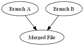
Graphical representation of a merge

Arguably the best way to rollback a commit in Subversion is to perform what they call a reverse-merge. In a normal merge, you take two versions of a file, compare them to figure out what’s different between them, and then create a new file containing the consensus content of both files (see picture to the right).

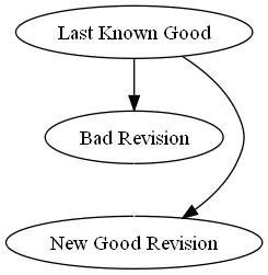
Graphical representation of a reverse merge

In a reverse-merge, you figure out what changes were made in a given revision, and then commit a new revision that reverts all of those changes back to the version before you committed your bad revision (see picture to the right), which means your bad revision will be simply skipped over as far as your comrades are concerned. Subversion provides a simple series of commands for this:

svn merge -c -{bad revision number} [{files to revert}]

Here’s how it works.

  1. The svn merge portion of the command basically tells Subversion you want to merge something. svn is the command-line tool to interact with a Subversion repository, and merge…well, you get the idea.
  2. -c -{bad revision number} tells Subversion that we want to work with the changes related to the revision numbered {bad revision number}. In this case, since we’re passing in a negative sign in front, we’re saying we want to remove those changes from the working directory. If you left out that negative sign, you’d actually pull the changes from that revision into the current working directory, which is usually only useful if you’re cherry-picking across branches. Whether that’s a good idea or not is left to the reader.
  3. [{files to revert}] are an optional list of files to undo changes in. Basically, if you pass in a list of files here, only those files will have their changes from revision–any other files changed in that revision will not be affected.

That’s pretty much it. Once you run that command (assuming there are no conflicts in your merge), you will be able to simply commit (with a helpful commit message, of course) and everything will be back to normal–your comrades in arms will be able to keep working without the overhead of your bad commit cluttering up their working environment, which is always a good thing.

Tar Pipe

This is the first in a series of posts I began this summer and only now have time to finish.

Every once in a while, I find myself needing to copy a large number of files from one Linux machine to another, ideally as fast as possible.  There are a lot of ways to do this, but the most common method usually goes something like this:

  • Tar everything up (with some form of compression if your network connection is slow).
  • (S)FTP/SCP  the file to the new server.
  • Move the file to the new location, making directories as needed.
  • Extract the tar file into the new directory.

This is all well and good, and it tends to work well in most cases–it’s just kind of laborious.  I prefer a simpler method that basically wraps everything up into a single step, affectionately known as a tar pipe.  The (admittedly somewhat complex) command follows.

  SRCDIR=  # fill in with your source directory
  DESTDIR= # fill in with your destination directory--note that your
           # uploaded directory will appear inside this one
  USER=    # fill in the your remote user name
  HOST=    # fill in with your remote host name
  tar -cvzf - $SRCDIR | ssh $USER@$HOST "mkdir -p $DESTDIR; tar -xz -C $DESTDIR

The variables are just to make things a little more easy to read (feel free to ignore them if you like), and I do recommend using a full path for the DESTDIR directory, but the basic process is ridiculously easy.  Here’s the breakdown on how the whole thing works.

  1. The tar -cvzf - $SRCDIR very obviously tars everything up, just like you normally would.  The key difference from the normal tar procedure is the fact that the “file” you’re creating with tar is actually sent to stdout (by the -f - option) instead of being written to the file system.  We’ll see why later.
  2. The | (pipe) passes everything on stdout on as stdin for the next command, just like normal.
  3. The ssh command is the fun part.
    1. We start an ssh session with $HOST as $USER.
    2. Once that’s established, we run two commands.
      1. mkdir -p $DESTDIR to make the destination directory, if needed.
      2. tar -xz -C $DESTDIR to untar something. What, we’re not sure yet.

What it untars is a bit of a mystery, as we don’t really tell it what it’s supposed to work on.  Or do we?  As it turns out, ssh passes whatever it receives on stdin on to the command it runs on the server.  I.e., all that stuff we just tar’red up gets passed along through the magic of piping from the local machine to the remote machine, then extracted on the fly once it gets to that machine.

You can see the benefit of this, I trust–instead of that whole four command process we detailed above, including manually logging into the remote server to actually extract the new file, we have one fairly simple command that handles taring, uploading, and extracting for us, with the added benefit of not requiring us to actually create any files we don’t have to create.  That’s kind of cool, right?

Note:  I’ve seen other implementations of the tar pipe, but this is the one I’ve used been using recently.  It’s worked for me on Red Hat 5, but your mileage may vary.

Résumé

CHAD BURRUS


113 N. Meridian St., Washington, Indiana 47501 (812) 783-9127;
[email protected]

Experience

Sentry Data Systems—Deerfield Beach, Florida
Software Developer: May 2011-Present

  • Served on an engineering board to address developer culture, standardize coding practices among
    projects and teams, and lead high-level software engineering decisions.

  • Managed our Jenkins server, including adding and updating builds as well as system-level
    configuration.

  • Managed releases of our SaaS products including actual rollouts with Capistrano and scripted database
    updates to Oracle.

  • Co-led a project to convert our Subversion repository to git.

  • Updated our Symfony 2.0 applications to use Symfony 2.1.

  • Integrated a Salesforce portal for customer support and help desk utilization.

  • Developed internal tools with PHP, PL/SQL, Ruby, and Twig.

School of Informatics and Computing, Indiana University—Bloomington, Indiana
Research Assistant: Jan. 2010-May 2011

  • Explored new association methods to compare metagenomic samples based on environmental data.

  • Wrote Python, R, and C++ code to analyze the differences in metagenomic samples including statistical
    tests and graph construction and development.

Sentry Data Systems—Deerfield Beach, Florida
Developer Intern: May 2010-Aug. 2010

  • Use PHP, PHPUnit, and PL/SQL to develop internal tools, including wrapping a set of PL/SQL classes
    with easy-to-use PHP classes.

  • Configure a Hudson build to ensure products stayed in good working order.

School of Informatics and Computing, Indiana University—Bloomington, Indiana
Associate Instructor, I101: Sept. 2009–Dec. 2009

  • Taught and graded weekly labs.

  • Assisted teaching additional lab sessions.

Cognitive Solutions, LLC.—Clearwater, Florida
System Developer: Sept. 2008–Aug. 2009

  • Developed both front-end and back-end components and features for a toy-tracking web application as
    part of a distributed development team.

LAT, Inc.—Marion, Indiana
Developer: Jan.–June 2006
Architect: June 2006–Aug. 2008

  • Designed and developed both front-end and back-end components and features for a wide range of web
    applications.

  • Served as technical lead for several projects, as well as occasional technical support and system
    administrator.

Education

Indiana University—Bloomington, Indiana
MS in Bioinformatics

  • Graduated May 2011 with an overall GPA of 3.95

Indiana Wesleyan University—Marion, Indiana
BS in Computer Science, Minor in Mathematics

  • Graduated April 2005 with an overall GPA of 3.75

Skills

Operating Systems:

  • Proficient with Linux (Ubuntu, Red Hat), Mac OS X, Windows 98/ME/XP/Vista/7

Computer Languages:

  • Proficient with CSS, HTML, Java, Javascript (including AJAX), LATEX, PHP, Python, XML, XSLT

  • Familiar with Ada, C, C++, Cobol, Matlab, Octave, Perl, R, Ruby, SQL (MySQL, PL/SQL, PostgreSQL,
    and SQL Server flavors)

Tools and Systems:

  • Proficient with Bash, CVS, git, jQuery, Komodo Edit, Mercurial, MySQL, Microsoft SQL Server,
    MooTools, PHPUnit, Scite, Subversion, Symfony 2, Twig, VIM

  • Familiar with Apache HTTP Server, Capistrano, Doctrine, Eclipse, Graphviz, Hudson/Jenkins, Joomla,
    Oracle

Achievements and Activities

ACM:

  • Student Member, 2003-2005.

  • Professional Member, 2005-Present.

IEEE Computer Society:

  • Student Member, 2005.

  • Associate Member, 2006-2009.

  • Graduate Student Member, 2009-2011.

  • Associate Member, 2011-Present.

Awarded Eagle Scout Rank, Boy Scouts of America (2000).

References

Available on request.

Mathematical glossary

Preface:  I’m not a mathematician, just a mere user of mathematics.  All the terms tend to confuse me, so here’s my personal glossary containing links to Wikipedia and MathWorld, a formal definition from one of those two places (which are usually overcomplicated if you’re just trying to use them), and my understanding of what each term means from a practical standpoint and/or an example of it that illustrates the main idea of the term.  This list should not be considered to be authoritative or complete, as I’m simply going to add terms as I run across them.  Feel free to correct me if you see any problems.

Linear Algebra

  1. Affine space – a point set with a faithful freely transitive vector space action for the vector space.  Essentially, it’s a normal vector space without an origin point, meaning we can treat any point we want as an origin during analysis (so long as we’re aware of the fact that we have no origin and will have to translate our “coordinates” if someone decides to move the origin on us).  (Wikipedia) (MathWorld)
  2. Eigenvalue – (no formal definition from either place except for in mathematical symbols I can’t copy) the amount by which an eigenvector changes when multiplied by its associated matrix. So, formally, if I have a square matrix A, eigenvector v, and scalar lambda, lambda is an eigenvalue if:

    Av = lambda v

    (Wikipedia) (MathWorld)

  3. Eigenvector – (no formal definition from either place except for in mathematical symbols I can’t copy) a vector that, when multiplied by a specific square matrix, changes only in magnitude, not in direction. So, formally, if I have a square matrix A, vector v, and scalar lambda (formally known as an eigenvalue), v is an eigenvector if:

    Av = lambda v

    (Wikipedia) (MathWorld)

  4. Vector space – a mathematical structure formed by a collection of vectors with an single point of origin.  An example would be normal Euclidean space. (Wikipedia) (MathWorld)

Statistical Basics

  1. Covariance – how much two variables change together.   (Wikipedia) (MathWorld)
  2. Cross-covariance (matrix) – sometimes used to refer to the covariance cov(XY) between two random vectors X and Y, in order to distinguish that concept from the “covariance” of a random vector X. So the key is that cross-variance refers to the covariance between a set of vectors, not the covariance within a single vector.  (Wikipedia) (MathWorld)
  3. Expected value (expectation or expectation value) – the integral of the random variable with respect to its probability measure.  Basically, it’s the value you expect to get out of  a function.  (Wikipedia) (MathWorld)
  4. Moment – a quantitative measure of the shape of a set of points.   (E.g., the “width” (the second moment) or “height” of the set of points, or the mean (the first moment) of the set of points.)  (Wikipedia) (MathWorld)
  5. Variance – a special case of covariance when the two variables are identical.  (I.e., when there is only one variable you’re really looking at.)  This measures how far values of the variable are from the mean of the variable.   (Wikipedia) (MathWorld)

Statistical Analysis Techniques

  1. Canonical correlation analysis (CCA–be careful, there are two of these) — a method of analysis that enables us to find linear combinations of two sets of correlated variables which have maximum correlation with each other.   This can be repeated up to n times, where n is the size of the smallest set.  (Wikipedia) (MathWorld)
  2. Principal component analysis (PCA) – a mathematical procedure that transforms a number of possibly correlated variables into a smaller number of uncorrelated variables called principal components.  You can think of this as taking a set of data and finding the best perspective to look at it, where the “best” perspective is the perspective that shows the most variation.  (Wikipedia) (MathWorld)

Topology

  1. Bijection (bijective map) – a function f from a set X to a set Y with the property that, for every y in Y, there is exactly one x in X such that f(x) = y.  Alternatively, f is bijective if it is a one-to-one correspondence between those sets. Basically, you have two sets, X and Y, and a function f that maps every value in X to a single value in Y.  That function f is the bijection.  (Wikipedia) (MathWorld — contains a great illustration if this is confusing)
  2. Diffeomorphic (diffeomorphism)-  an isomorphism in the category of smooth manifolds. It is an invertible function that maps one differentiable manifold to another, such that both the function and its inverse are smooth. (Wikipedia) (MathWorld)
  3. Embedding – one instance of some mathematical structure (call it X) contained within another instance (call it Y) where X maps to Y via an injective and structure-preserving map f.  Examples include the natural numbers (X) within the integers (Y), or the integers (X) within the rational numbers (Y).  This is similar to, but distinct from, the idea of a subset.  (Embedding seems to be more general.)  (Wikipedia) (MathWorld)
  4. Homomorphism –  a structure-preserving map between two algebraic structures (such as groups, rings, or vector spaces). (Wikipedia) (MathWorld)
  5. Injective – a function that preserves distinctness: it never maps distinct elements of its domain to the same element of its codomain.  (Wikipedia) (MathWorld)
  6. Isomorphism – a bijective map f such that both f and its inverse f −1 are homomorphisms. (Wikipedia) (MathWorld)
  7. Manifold – a mathematical space that on a small enough scale resembles the Euclidean space of a specific dimension.  A line is a one-dimensional manifold since if you look at a small area around any given point of a line, that area resembles one-dimensional space.  Likewise, a sphere (specifically the surface, not the volume), is a tw0-dimensional manifold since that surface can be represented by a set of two-dimensional maps, according to Wikipedia, though to me that doesn’t quite make sense.  You can indeed represent a sphere as two-dimensional maps (check out your handy road map if you don’t believe me), but not without distorting the map somehow, usually via some sort of projection or a non-rectangular drawing.  (Wikipedia) (MathWorld)
  8. Morphism – an abstraction derived from structure-preserving mappings between two mathematical structures. (Wikipedia) (MathWorld)

RAMMCAP: CD-HIT and ORF_FINDER

This is the second part of a series of posts on the RAMMCAP suite of bioinformatics tools.

Last time, we left off with a freshly compiled version of RAMMCAP ready for testing.  Like last time, we’ll start with the README in the current directory, which is the rammcap directory inside the main directory (named RAMMCAP-20091106 in my case) from the RAMMCAP download.

The new README has its own test script, so I’m going to follow this one. The first thing to run is the CD-HIT-EST program.

CD-HIT-EST

The CD-HIT-EST program is the clustering program. It takes in a FASTA-formatted file and clusters that data according to a greedy algorithm that uses simple word counting and indexing to help speed things up considerably. Basically, it:

  1. Sorts the sequences from longest to shortest.
  2. Begins clustering:
    1. Compare the current sequence to the list of known clusters.
      1. If it matches an existing cluster, it is added to that cluster and made the “representative” sequence for that cluster if it is longer than the existing “representative” sequence.
      2. If it doesn’t match an existing cluster, a new cluster is made with this sequence as the representative sequence.
    2. Repeat until all the sequences are clustered.

(None of which I knew at the time I ran this for the first time, but it’s information that makes sense here.)

I pull out the really long test command (written below), prepare myself, and hit Enter. It takes a long time to complete.

../cd-hit/cdhit-est -i testdb -o testdb_95 -M 50 -B 1 -d 0 -n 10 
     -l 11 -r 1 -p 1 -g 1 -G 0 -c 0.95 -aS 0.8 > testdb_95.log

While that’s going, here’s what that command means:

  • ../cd-hit/cd-hit-est – use the CD-HIT-EST command, which is the CD-HIT command for DNA/RNA comparison tasks. The original CD-HIT was written for protein comparison.
  • -i testdb – use the testdb file as the input file. This file is a FASTA file with 1,000,000 sequences at most 361 bases long pulled from various metagenomic samples by the author.
  • -o testdb_95 – write the output to a file called testdb_95
  • -M 50 – I have 50 MB of RAM free (which I don’t think really makes sense, but that’s what the README says)–turns out it’s actually the maximum available memory, not the amount of free memory according to the rest of the documentation.
  • -B 1 – sequences are stored on the hard drive (1) instead of in RAM (0)
  • -d 0 – The length of the description in .clster file. Since it’s 0, it just takes the FASTA sequence description up to the first space.
  • -n 10 – the word length
  • -l 11 – length of the throw_away_sequences
  • -r 1 – compare both strands of DNA
  • -p 1 – print the alignment overlap in the .clstr file (if 0, it’s not printed)
  • -g 1 – clusters the strings into the most similar cluster, not the first one CD HIT finds, which is the default (0).
  • -G 0 – don’t use global sequence identity, i.e., treat each input sequence individually when calculating identity.
  • -c 0.95 – cluster at 95% sequence identity
  • -aS 0.8 – alignment coverage for the shorter sequence. In this case, it means that the alignment between the longer and shorter sequence must cover at least 80% of the shorter sequence.
  • > testdb_95.log – write the standard output to the testdb_95.log file
  • There are other options available, which I’m not going to go into much for right now.

Long story short, it takes around 200 minutes to complete its test data processing. That’s roughly 3 hours and 20 minutes, which I think is pretty long for a test, though I did limit the amount of memory it could use to 50 MB–upping that limit will probably speed things up substantially, but according to what I read in the README I couldn’t. In retrospect, though, I think upping the limit is just fine, especially with the information I’m reading in the other files. (UPDATE: Upping the memory limit to 400MB, the default, drops the execution time down to about 67 minutes. Eight fold memory increase, three fold time decrease–not great, but not too shabby.)

ORF_FINDER

The next program to run is the ORF_FINDER. This program apparently is a program to scan the sequences for ORFs (not surprising given the name), which are what most people mean when they talk about their “genes” and their DNA (kind of).

../orf_finder/orf_finder -l 30 -L 30 -t 11  -i testdb -o testorf

This command takes far fewer options.

  • ../orf_finder/orf_finder – runs the orf_finder command.
  • -l 30 – the minimal length of the ORF.
  • -L 30 – the minimal length of the ORF between stop codons. I’m not sure exactly how this differs from the -l option. Maybe you need to move at least 30 bases past the end of the previous stop codon before starting to look for another stop codon?
  • -t 11 – Translation table?. Again, not sure what this represents.
  • -i testdb – Use the testdb file as input.
  • -o testorf – Write the output to the testorf file.
  • Again, there are other options I’m not going to talk about much.

In addition to having far fewer options, ORF_FINDER takes far less time to execute. Roughly a minute and a half on the same dataset, which is a pretty huge upgrade. ORF finding is a much simpler task than sequence clustering, obviously. Now for the fun part–clustering the ORFs with the real CD-HIT program.

CD-HIT

Now, CD-HIT works basically the same way that CD-HIT-EST does, except it scans for amino acids instead of nucleotides. The full commands I’m running are:

../cd-hit/cdhit -i testorf -o testorf_95 -M 400 -d 0 -n 5 -p 1 
     -g 1 -G 0 -c 0.95 -aS 0.8 > testorf_95.log
../cd-hit/cdhit -i testorf_95 -o testorf_60 -M 400 -d 0 -n 4 -p 1 
     -g 1 -G 0 -c 0.60 -aS 0.8 > testorf_60.log
../cd-hit/clstr_rev.pl testorf_95.clstr testorf_60.clstr 
     > testorf_60full.clstr

It has much the same options as CD-HIT-EST, so I’m not going go into a huge amount of detail on those. Instead, notice how I’m going to:

  1. Cluster the ORFS at 95% identity.
  2. Re-cluster the ORFs with less stringent criteria (60% identity and a shorter word length) to help cluster the non-redundant sequences.
  3. Combine the two clustering runs into a single cluster file.

Running things this way (according to the documentation) can help generate a sort of hierarchical structure of clusters. This makes sense, since the ones at 95% identity at the very least are closely related and may actually be redundant sequences while those at 60% are more distant relatives and may be homologs from divergent species or something similar.

The first run of CD-HIT took around 98 minutes, roughly an extra half an hour than just clustering the sequences as a whole. I’m guessing that since the ORFs are more similar to each other than just the sequences as a whole that they take longer to cluster.

The second run of CD-HIT took around 235 minutes, probably because the less stringent criteria took longer to process. Combining the two cluster files only took around 15 seconds, so at least that’s an easy task.

That takes care of the basic tools included with RAMMCAP.  I’ll explore some of the graphical tools in a later post.

RAMMCAP: Introduction, Download, and Install

This is the first part of a series of posts on the RAMMCAP suite of bioinformatics tools.

The Rapid Analysis of Multiple Metagenomes with a Clustering and Annotation Pipeline (RAMMCAP) is a tool used for analysis of metagenomic data. What it does is try to cluster and functionally annotate a set of metagenomic data, which means it takes the data, groups like pieces of data together into clusters, and then tries to figure out what the various clusters do. It’s made up of several tools, only two of which I’ve actually used and I’ll talk about later. Camera, the organization behind RAMMCAP, provides a web service where you can use RAMMCAP without installing it, but it has data limits that I’ll break very easily with my datasets plus they require registration, which seems non-functional right now (at least, I can’t get a new account set up and I’ve tried several times over the course of the last few days). So, I downloaded it a few weeks ago and worked on getting it to run over the course of several days.  This post, and the others in this series, is a record of that process, including some initial miss-steps.  If you have any questions or see other places where I stepped wrongly, leave a comment and let me know.

First Impressions

First off, the RAMMCAP download (found on the page linked above) is huge–the source code alone was a roughly 760 MB download, which extracts to around 3 gigs. That three gigs might contain some duplicate data–the folder structure is pretty disorganized and a casual glance shows a lot of folders with the same names. There are a lot of symlinks, though, so I could be wrong there. (The more I see, the more I’m convinced I’m right, though.)

Second, it looks like the source bundled a bunch of tools along with the main RAMMCAP code, including versions of BLAST, HMMER, and Metagene. That added a lot to the bulk of the download (roughly 450 MB). There’s also a huge amount of data here, including a version of the Pfam and TIGRFAM libraries (772 and 444 MB, respectively), and a couple other tools I haven’t heard of before that might be part of RAMMCAP.

Compiling, Phase 1

The README file in the main directory contains basic information on how to compile some of the tools including CD-HIT, ORF_FINDER, and CD-HIT-454, as well as the HMMERHEAD extension to the HMMER, which is optional. The instructions are pretty basic–just do the standard “make clean;make” and things should be good. I wrote a little build script to handle this, just in case I need to do this again for some reason. Everything seems to build fine with the exception of HMMERHEAD, but I’m just going to ignore that for now. Time for testing this puppy out.

Testing, Phase 1

The README indicates that there should be an examples folder somewhere with some basic test data I can use, but I don’t see it anywhere. Looking around…not seeing it. Turns out, it’s inside the rammcap directory inside the main directory.

Compiling, Phase 2

Inside the rammcap directory, I find a new README with some major differences from the one outside this directory, plus what looks like symlinks with the same names as some of the directories outside. Looks like they point to the same directories as the other ones, but I’ll recompile things, anyway, just in case. Good thing I wrote that build script.

Except that the build instructions aren’t the same–I don’t have to build CD-HIT-454, but I do need to make sure gnuplot and ImageMagick are installed. They are, which is good, because I’d either have to contact one of the tech guys to install it on this machine or I’d have to install it to my user directory, which I’ve done with several tools I need or don’t want to do without. Once I pull out that CD-HIT-454 reference, the build works fine.

Since my second round of testing was a much larger task, I’ll leave that for a later post.

Linux Screen Command

Normally, when you log into a remote server via SSH, you get one command prompt and so there’s essentially only one thing you can do at a time without a lot of extra hassle.  However, most of the time I (and presumably others like me) need to do lots of things, potentially in different directories spread out all over the place.  Since switching back and forth between directories all the time is only one of those hassles I mentioned, more often than not I end up with multiple SSH connections to the same server.

Like a couple days ago–I had a connection open to edit my files, one to handle my version control (Mercurial, if you’re curious–more on that later), and one to keep tabs on my data.  Juggling multiple connections like that is easy in a GUI–a couple of quick “Alt-Tabs” and you’ve gone from your editor to your data directory to your version control and back again.  However, all those connections can eat up your bandwidth and many other less-than-fun things, especially when there’s a handy little tool around to do the same kind of thing built right in to the Linux (and presumably other Unix-like OS’s)–the screen command.

The screen command essentially allows you to create multiple “windows” or “screens” you can use within the same connection.  You get multiple command prompts you can work with, and a handy keyboard shortcut similar to but slightly less convenient than “Alt-Tab” to switch between your “screens”.  Another benefit to using screen is that your sessions can survive across SSH sessions–you can disconnect from your screen, log off the server, go away to do something more fun for a couple hours, log back in, and resume right where you left off–same environmental variables, same directory, same command history, etc.  You can even use screen to run long-running commands (say, a command that takes hours or days to run) without having to stay logged in the whole time.  Pretty cool, huh?

You can get most of the information you need to use the screen command effectively out of the man page (this one’s not bad), but I’ll summarize the pieces I find most useful here.

First off, you need to create a new screen, ideally with a name, so you can resume them more easily later and not have to remember a weird id number.  To make a screen named “screenTest” for example, run the following command:

     screen -S screenTest

You should be switched over to a new command prompt and see something like “[screen 0: bash]” in your SSH session’s title, assuming your SSH client supports that kind of change.

The next thing you need to know is how to create what I call a “subscreen,” though I don’t think that’s an official term.  (I’d run a simple command like “ls” now so you can tell the difference between your “subscreens.”)  Hit CTRL+A, release them both, and hit C.  Once again, you should see a new command prompt and something like “[screen 1: bash]” in your window’s title.  Switch back and forth between your “subscreens” by hitting CTRL+A twice just to see that you can, or until you’re convinced there’s a difference between the two.  If you have more than two subscreens, you need to know about a couple more things about subscreen navigation:

  1. CTRL+A twice navigates to the most recently used subscreen.
  2. CTRL+A, N navigates to the “next” subscreen in your list of subscreens.
  3. CTRL+A, P navigates to the “previous” subscreen in your list.
  4. CTRL+A, 0 navigates to the screen numbered 0.  You can use any number between 0-9 for the same effect.
  5. CTRL+A, ” opens up a list of the screens you can move between.
  6. CTRL+A, ‘ prompts you for a screen number and allows you to bounce straight to that screen.

Now, it’s time to drop out of your screens as if you were going to log out.  Hit CTRL+A followed by D, and you should be “detached” from your current screen.  You’ll have returned to your original command prompt, with a little “[detached]” message right after your screen command.

Let’s pretend you wandered away from your computer and came back, ready to start work again.  You need to resume your previous session, so run this command.

     screen -r screenTest

Voilà!  Your screen should open up, just like it was when you detached from it earlier (unless you were running a long command, in which case the output is probably different, but that’s beside the point).  Having fun yet?

One more thing that you might need to know is how to connect to a screen that’s already attached somewhere else, or that didn’t get detached properly somehow (I’ve had it happen once or twice).  This one’s pretty obvious, as well.

     screen -d screenTest

If you pass the “-r” flag to that command, as well, you will detach the other session and connect to it yourself, which can be helpful if you’re moving between computers or something like that.

When it’s time to nuke a screen completely (like if you were a smart person and set up separate screens for each project you’re working on, and just finished one of them), getting rid of it is really easy.  Attach to it, and hit CTRL+D until you close out all of the subscreens.  Be careful you don’t nuke your real session, though, because it’s really easy to do.

One caveat–if you use screen a lot, get used to piping things through less, since the scroll bar of your window will do strange things while you’re running screen.

Ok, that takes care of the basics.  Have fun!